1. Freezing cycles tolerance
Matteo Vecchi
2023-01-10
Last updated: 2023-01-10
Checks: 6 1
Knit directory: freezing_cycles/
This reproducible R Markdown analysis was created with workflowr (version 1.7.0). The Checks tab describes the reproducibility checks that were applied when the results were created. The Past versions tab lists the development history.
The R Markdown file has unstaged changes. To know which version of
the R Markdown file created these results, you’ll want to first commit
it to the Git repo. If you’re still working on the analysis, you can
ignore this warning. When you’re finished, you can run
wflow_publish to commit the R Markdown file and build the
HTML.
Great job! The global environment was empty. Objects defined in the global environment can affect the analysis in your R Markdown file in unknown ways. For reproduciblity it’s best to always run the code in an empty environment.
The command set.seed(20220415) was run prior to running
the code in the R Markdown file. Setting a seed ensures that any results
that rely on randomness, e.g. subsampling or permutations, are
reproducible.
Great job! Recording the operating system, R version, and package versions is critical for reproducibility.
Nice! There were no cached chunks for this analysis, so you can be confident that you successfully produced the results during this run.
Great job! Using relative paths to the files within your workflowr project makes it easier to run your code on other machines.
Great! You are using Git for version control. Tracking code development and connecting the code version to the results is critical for reproducibility.
The results in this page were generated with repository version ed0e131. See the Past versions tab to see a history of the changes made to the R Markdown and HTML files.
Note that you need to be careful to ensure that all relevant files for
the analysis have been committed to Git prior to generating the results
(you can use wflow_publish or
wflow_git_commit). workflowr only checks the R Markdown
file, but you know if there are other scripts or data files that it
depends on. Below is the status of the Git repository when the results
were generated:
Ignored files:
    Ignored:    .Rhistory
    Ignored:    .Rproj.user/
    Ignored:    analysis/site_libs/

Untracked files:
    Untracked:  analysis/2.freezing_vs_environment.Rmd
    Untracked:  data/tree.nwk
    Untracked:  output/tree_Cycles.pdf

Unstaged changes:
    Deleted:    .DS_Store
    Modified:   analysis/0.data.Rmd
    Modified:   analysis/1.freezing_cycles_tolerance.Rmd
    Deleted:    analysis/2.long_freezing_vs_cycles.Rmd
    Deleted:    analysis/3.freezing_vs_environment.Rmd
    Modified:   analysis/index.Rmd
    Modified:   code/model.txt
    Deleted:    data/.DS_Store
    Modified:   data/data_freezing.xlsx
    Modified:   data/mixedmonths_data.txt
    Deleted:    data/tree.nex
    Modified:   freezing_tardigrades.Rproj
    Deleted:    output/M_vs_plong_plot.svg
    Modified:   output/means_cycles.txt
    Modified:   output/mod.env.rds
    Modified:   output/model_fit.env.pdf
    Deleted:    output/plot_mod_fitenv.pdf
    Deleted:    output/tree_Cycles.svg
Note that any generated files, e.g. HTML, png, CSS, etc., are not included in this status report because it is ok for generated content to have uncommitted changes.
There are no past versions. Publish this analysis with
wflow_publish() to start tracking its development.
library(tidyverse)
library(dplyr)
library(readxl)  # To read from excel files
library(R2jags)
library(ggplot2)
library(patchwork)
library(DT)
library(xfun)          # Download file from html report
library(ape)
library(phytools)
library(svglite)
library(Hmisc)
library(ggtree)
1. Freezing-thaw cycles
the Model
In this part we are going to estimate the number of cycles needed for each species to kill 50% of the individuals. To do so we are gonna fit the cumulative function of a discrete Weibull distribution, and then estimate its x value (# of cycles) at y = 0.5 (half of animals dead). The function we are gonna use to estimate the probability of an individual be dead at each cycle is:
\[ p = 1- e^{-(\frac{t+1}{\alpha})^\beta} \] We are however, more interested to the number of cycles needed to kill 50% of individuals (M). M will be calculated from the \(\alpha\) and \(\beta\) parameters as follows: \[ M = \alpha * (-log(0.5)^\frac{1}{\beta})-1\] Based on these two equations, we reparametrize the cumulative discrete Weibull distribution to predict the alive individuals (instead than the dead ones in its origigan formulation) and to use M instead than \(\alpha\). This reparametrization has two advantages: 1) we can easily constrain with priors M to be positive (it makes biologically sense as there cannot be a negative number of freezing cycles) ad 2) we will obtain as output of the models M directly without the need of processing the posteriors too much. The reparametrized function used in the model will be: \[ p = e^{-(\frac{(t+1)*(-log(0.5)^\frac{1}{\beta})}{1 + M})^\beta} \]
The two parameters to be estimated will be \(\alpha\) and \(\beta\), whereas p will be fitted
for each animal at each cycle trough a Bernoulli distribution as
follows:
\[ alive \ animals \sim DBernoulli(p)
\]
Dataset subsetting
We are going to estimate \(\alpha\) and \(\beta\) with a Bayesian approach using the software JAGS trough the R package “R2jags”.
- As in some data points the well didn´t freeze during the permanence
at -7C, we are going to test the model on 3 different version of the
dataset to test if those points are problematic and should be excluded
from analysis or if they don´t change the result:
- Dataset da1: the original dataset with all the points.
- Dataset da2: only the datapoints (individual * cycle) when a well didn´t freeze are excluded.
- Dataset da3: all individuals that didn´t freeze at least once are excluded.
# Load the data
data_cycles = read_xlsx("./data/data_freezing.xlsx", sheet = "data_cycles")
species_abbrev = read_xlsx("./data/data_freezing.xlsx", sheet = "species_abbrev")

# Subset the data
da1 = data_cycles %>% gather("cycle","alive",2:9)
da2 = data_cycles %>% gather("cycle","alive",2:9) %>% subset(when != cycle)
da3 = data_cycles %>% gather("cycle","alive",2:9) %>% subset(unfrozen == 0)
The first dataset (da1) has 4800 data points, the second (da2) has 4752, whereas da3 has 4416 data points, so even with the harshest data subsetting (da3) we don´t loose many data points.
JAGS data
We prepare the three data objects for JAGS, each for every susbet version of the dataset.
data.jags.da1 = list(alive = as.integer(da1$alive),                        # if an animal was alive
                 cycle = as.integer(da1$cycle),                            # cycle number
                 species_num = as.numeric(as.factor(da1$species_code)),    # what species is that animal
                 Nsp = length(unique(da1$species_code)))                   # number of species (to allow the model to loop trought species)

data.jags.da2 = list(alive = as.integer(da2$alive),
                 cycle = as.integer(da2$cycle),
                 species_num = as.numeric(as.factor(da2$species_code)),
                 Nsp = length(unique(da2$species_code)))

data.jags.da3 = list(alive = as.integer(da3$alive),
                 cycle = as.integer(da3$cycle),
                 species_num = as.numeric(as.factor(da3$species_code)),
                 Nsp = length(unique(da3$species_code)))
JAGS model
The model function for JAGS is the same for the three dataset, so their resuts will be directly comparable.
model.jags.da = function(){

  # Priors
  for (sp in 1:Nsp) {        # we estimate M and beta separately for each species
    beta[sp] ~ dexp(0.1)     # very low informative prior bound to be >0
    M[sp] ~ dexp(0.1)        # very low informative prior bound to be >0
  }


  # Likelihood
  for (i in 1:length(alive)){


    numerator[i] <- (cycle[i]+1)*((-log(0.5))^(1/beta[species_num[i]]))
    p_alive[i] <- exp(-((numerator[i]/(1+M[species_num[i]]))^(beta[species_num[i]])))

    p_regularized[i] <- ifelse(p_alive[i] == 0, 0.00001, ifelse(p_alive[i] == 1, 0.99999, p_alive[i])) # This is to avoid the model to crash when p is exactly 0 or 1

    alive[i] ~ dbern(p_regularized[i])

  }

}
Run the JAGS models
As the models takes long time to run, the results are saved as RDS files. If the models has been already run in the working directory, instead of rerun them, they will be loaded from memory.
# Model da1
ifelse("mod.da1.rds" %in% list.files("./output"),{mod.da1 = readRDS("./output/mod.da1.rds")},{

  mod.da1 = jags(data = data.jags.da1, parameters.to.save =  c("M"), model.file = model.jags.da, n.iter = 10000)
write_rds(mod.da1, file="./output/mod.da1.rds")

})


# Model da2
ifelse("mod.da2.rds" %in% list.files("./output"),{mod.da2 = readRDS("./output/mod.da2.rds")},{

  mod.da2 = jags(data = data.jags.da2, parameters.to.save =  c("alpha","beta"), model.file = model.jags, n.iter = 1000000)
write_rds(mod.da2, file="./output/mod.da2.rds")

})


# Model da3
ifelse("mod.da3.rds" %in% list.files("./output"),{mod.da3 = readRDS("./output/mod.da3.rds")},{

  mod.da3 = jags(data = data.jags.da3, parameters.to.save =  c("alpha","beta"), model.file = model.jags, n.iter = 1000000)
write_rds(mod.da3, file="./output/mod.da3.rds")

})
Plot the models estimates
We are now going to plot side by side the M estimated for each model (divided by species) to check if different data subsetting strategies to deal with the issue of some wells not freezing affect the M estimates.
# First we create a table to code back the species numebrs used in the models to their species names
lev_to_num = data.frame(number = 1:length(levels(as.factor(data_cycles$species_code))),
                        species_code =  levels(as.factor(data_cycles$species_code))) %>% merge(species_abbrev)

# We then create a function to extract the species number from the variable names in the model outputs
extract.number = function(x){as.numeric(gsub(".*?([0-9]+).*", "\\1", x))}

# Now we extract the chains and do some cleaning of the data to have them ready for plotting
chains.da1 = data.frame(do.call(rbind, as.mcmc(mod.da1))) %>% dplyr::select(!deviance) %>% gather("species_var","M") %>%
  mutate(number = extract.number(species_var), model = rep("da1",nrow(.))) %>% merge(lev_to_num)

chains.da2 = data.frame(do.call(rbind, as.mcmc(mod.da2))) %>% dplyr::select(!deviance) %>% gather("species_var","M") %>%
  mutate(number = extract.number(species_var), model = rep("da2",nrow(.))) %>% merge(lev_to_num)

chains.da3 = data.frame(do.call(rbind, as.mcmc(mod.da3))) %>% dplyr::select(!deviance) %>% gather("species_var","M") %>%
  mutate(number = extract.number(species_var), model = rep("da3",nrow(.))) %>% merge(lev_to_num)

chains_all = rbind(chains.da1, chains.da2,chains.da3)

# Plotting
ggplot(chains_all)+
  theme_bw()+
  geom_violin(aes(x=model, y=M, fill=model), alpha = 0.50, scale = "width", col = NA, show.legend = F)+
  facet_wrap(.~species, scales="free_y")+
  stat_summary(aes(x=model, y=M, group=model),fun=median, colour="black", geom="point", size = 3)+
  stat_summary(aes(x=model, y=M, group=model),fun.data=median_hilow, colour="black", geom="linerange")+
  expand_limits(y=0) + ylab("# of cycles to death of 50% of individuals") + xlab("Model")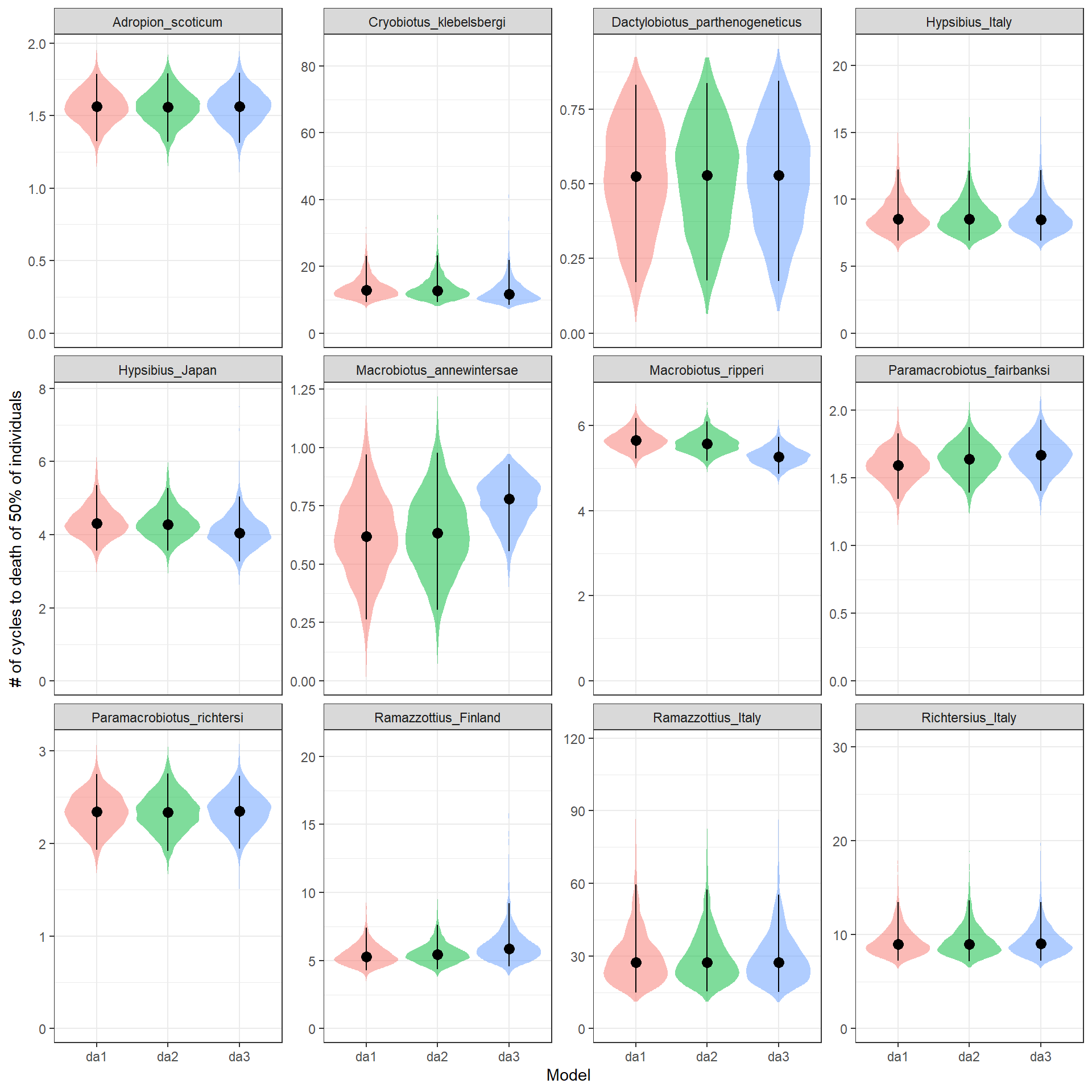
| Version | Author | Date |
|---|---|---|
| df35b09 | Matteo Vecchi | 2022-04-21 |
For almost all species the estimated of the different models are almost identical. Only form Marobiotus ripperi and Macrobiotus annewintersae they look different in the model da3, howevere they still overlap with the estimated of da1 and da2 that look very similar to each other. Given the small influence of the data points where the well didn’t freeze, we will continue the analysis by keeping the most complete model, aka da1.
Now we can calculate the mean estimates of the number of cycles to death of 50% of individuals for each species
means_cycles = aggregate(chains.da1$M, by=list(chains.da1$species_code),
                         FUN=function(x){c(mean(x),quantile(x,probs = c(0.025, 0.975)))})
means_cycles = data.frame(means_cycles$Group.1,means_cycles$x)
colnames(means_cycles) = c("species_code", "M","low95","high95")
means_cycles = merge(species_abbrev, means_cycles)
means_cycles[,2:5]
species M low95 high95
1 Adropion_scoticum 1.5619741 1.3248099 1.7872009
2 Dactylobiotus_parthenogeneticus 0.5197142 0.1712878 0.8317143
3 Hypsibius_Italy 8.7911024 6.8981101 12.2176230
4 Hypsibius_Japan 4.3498234 3.5606402 5.3589581
5 Cryobiotus_klebelsbergi 13.7464415 9.3153940 23.0414070
6 Macrobiotus_annewintersae 0.6210363 0.2643385 0.9710929
7 Macrobiotus_ripperi 5.6631451 5.2249238 6.1764720
8 Paramacrobiotus_fairbanksi 1.5904498 1.3439225 1.8266957
9 Paramacrobiotus_richtersi 2.3420092 1.9273249 2.7480961
10 Richtersius_Italy 9.3578652 7.2181733 13.4528368
11 Ramazzottius_Italy 29.7291315 14.9947610 59.5875491
12 Ramazzottius_Finland 5.4514370 4.2608211 7.4319653write.table(means_cycles, "./output/means_cycles.txt")Plot the estimates against phylogeny
chains_toplot = chains.da1[,c(3,6)]

# load the tree
tree = read.tree("./data/tree.nwk")
tree = root(tree,"Milnesium_variefidum")
tree = chronos(tree)
tree = drop.tip(tree, tip = tree$tip.label[!(tree$tip.label %in% unique(chains.da1$species))])
class(tree) = "phylo"


#this part gets the order of the tip labels as plotted in ggtree
d = fortify(tree)
d = subset(d, isTip)
tips.order = rev(with(d, label[order(y, decreasing=T)]))

#reorder the species
chains_toplot = chains_toplot[chains_toplot$species %in% tips.order,]
chains_toplot$species = factor(chains_toplot$species, levels = tips.order)


#make the plot
treeplot = ggtree(tree,size=1) + # plot tree topology
  theme_bw()+
  theme(panel.grid.major = element_blank(),
        panel.grid.minor = element_blank(),
        axis.title=element_blank(),
        axis.text=element_blank(),
        axis.ticks=element_blank(),panel.border = element_blank())

T50plot = ggplot(chains_toplot)+
  theme_bw()+
  geom_violin(aes(x=species, y=M+1), alpha=0.5, scale="width", show.legend=T, color="NA", fill="lightblue")+
  #scale_fill_viridis_c()+
  scale_y_continuous(trans="log",breaks = c(1,2,6,11,21,41,81), labels =c(0,1,5,10,20,40,80))+
  #scale_y_continuous(trans="sqrt",breaks = seq(0,80,5), labels = seq(0,80,5))+
  #scale_y_continuous(trans="log2",breaks = seq(0,80,5)+1, labels =seq(0,80,5))+
  scale_fill_gradient2(high="#FF6699", mid="#CC99FF", low="#3399FF", na.value = "grey50",midpoint=0)+
  stat_summary(aes(x=species, y=M+1),fun=median, colour="black", geom="point", size = 3)+
  stat_summary(aes(x=species, y=M+1),fun.data=median_hilow, colour="black", geom="linerange")+
  xlab("")+ylab("")+coord_flip()+
  scale_x_discrete(position = "top")+
  theme(panel.grid.major.y = element_blank(), panel.grid.minor = element_blank(),panel.border =    element_blank())


(treeplot|T50plot) +  plot_layout(widths = c(1,2))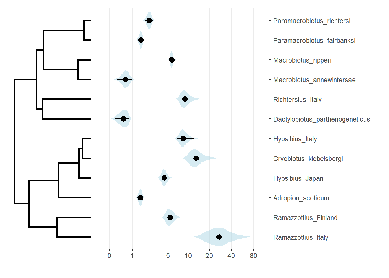
| Version | Author | Date |
|---|---|---|
| df35b09 | Matteo Vecchi | 2022-04-21 |
ggsave("./output/tree_Cycles.pdf")Download the plot in pdf format
Download tree_Cycles.pdfPhylogenetic signal tests
We can test the estimated resistance to repeated freezing cycles (as # of cycles to death of 50% of individuals) for phylogenetic signal.
# We already have the mean estimates for the # of cycles, however we can calculate their se to improve the phylogenetic signal estimation
se_cycles = aggregate(chains.da1$M, by=list(chains.da1$species_code), FUN=function(x) sqrt(var(x) / length(x)))
colnames(se_cycles) = c("species_code", "M")
se_cycles = merge(species_abbrev, se_cycles)

# Transform them to vectors for the phylosig function
M_mean = means_cycles$M
names(M_mean) = means_cycles$species

M_se = se_cycles$M
names(M_se) = se_cycles$species

# Keep only taxa present both in tree and data vectors
M_mean = M_mean[names(M_mean) %in% tree$tip.label]
M_se = M_se[names(M_se) %in% tree$tip.label]

K_phylosig = phylosig(tree, M_mean , method="K", test=TRUE, se = M_se)
lambda_phylosig = phylosig(tree, M_mean , method="lambda", test=TRUE, se = M_se)


K_phylosig
Phylogenetic signal K : 0.652263
MLE(sig2) : 126.283
logL(sig2) : -41.7566
P-value (based on 1000 randomizations) : 0.145
lambda_phylosig
Phylogenetic signal lambda : 0.215301
logL(lambda) : -41.7542
MLE(sig2) : 63.0272
LR(lambda=0) : 0.0875663
P-value (based on LR test) : 0.767294
It seems there is no phylogenetic signal (Bloombers´s K) in the resistance to freeze-thaw cycles, however the sample is low (12 species), so those results should be taken cautiously.
sessionInfo()R version 4.2.1 (2022-06-23 ucrt)
Platform: x86_64-w64-mingw32/x64 (64-bit)
Running under: Windows 10 x64 (build 19044)
Matrix products: default
locale:
[1] LC_COLLATE=English_United Kingdom.utf8
[2] LC_CTYPE=English_United Kingdom.utf8
[3] LC_MONETARY=English_United Kingdom.utf8
[4] LC_NUMERIC=C
[5] LC_TIME=English_United Kingdom.utf8
attached base packages:
[1] stats graphics grDevices utils datasets methods base
other attached packages:
[1] ggtree_3.3.1 Hmisc_4.7-1 Formula_1.2-4 survival_3.4-0
[5] lattice_0.20-45 svglite_2.1.0 phytools_1.2-0 maps_3.4.1
[9] ape_5.6-2 xfun_0.34 DT_0.26 patchwork_1.1.2
[13] R2jags_0.7-1 rjags_4-13 coda_0.19-4 readxl_1.4.1
[17] forcats_0.5.2 stringr_1.4.1 dplyr_1.0.10 purrr_0.3.5
[21] readr_2.1.3 tidyr_1.2.1 tibble_3.1.8 ggplot2_3.4.0
[25] tidyverse_1.3.2
loaded via a namespace (and not attached):
[1] backports_1.4.1 fastmatch_1.1-3 workflowr_1.7.0
[4] systemfonts_1.0.4 igraph_1.3.5 lazyeval_0.2.2
[7] splines_4.2.1 digest_0.6.30 yulab.utils_0.0.5
[10] htmltools_0.5.3 fansi_1.0.3 magrittr_2.0.3
[13] checkmate_2.1.0 optimParallel_1.0-2 googlesheets4_1.0.1
[16] cluster_2.1.4 tzdb_0.3.0 modelr_0.1.10
[19] timechange_0.1.1 jpeg_0.1-9 colorspace_2.0-3
[22] rvest_1.0.3 textshaping_0.3.6 haven_2.5.1
[25] crayon_1.5.2 jsonlite_1.8.3 phangorn_2.10.0
[28] glue_1.6.2 gtable_0.3.1 gargle_1.2.1
[31] abind_1.4-5 scales_1.2.1 DBI_1.1.3
[34] Rcpp_1.0.9 plotrix_3.8-2 htmlTable_2.4.1
[37] gridGraphics_0.5-1 tidytree_0.4.1 foreign_0.8-83
[40] htmlwidgets_1.5.4 httr_1.4.4 RColorBrewer_1.1-3
[43] ellipsis_0.3.2 pkgconfig_2.0.3 farver_2.1.1
[46] nnet_7.3-18 sass_0.4.2 dbplyr_2.2.1
[49] deldir_1.0-6 utf8_1.2.2 ggplotify_0.1.0
[52] tidyselect_1.2.0 labeling_0.4.2 rlang_1.0.6
[55] later_1.3.0 munsell_0.5.0 cellranger_1.1.0
[58] tools_4.2.1 cachem_1.0.6 cli_3.4.1
[61] generics_0.1.3 broom_1.0.1 evaluate_0.18
[64] fastmap_1.1.0 yaml_2.3.6 ragg_1.2.4
[67] knitr_1.41 fs_1.5.2 nlme_3.1-160
[70] mime_0.12 whisker_0.4 aplot_0.1.8
[73] xml2_1.3.3 compiler_4.2.1 rstudioapi_0.14
[76] png_0.1-7 reprex_2.0.2 treeio_1.19.1.900
[79] clusterGeneration_1.3.7 bslib_0.4.1 stringi_1.7.8
[82] highr_0.9 Matrix_1.5-3 vctrs_0.5.0
[85] pillar_1.8.1 lifecycle_1.0.3 combinat_0.0-8
[88] jquerylib_0.1.4 data.table_1.14.4 httpuv_1.6.6
[91] R2WinBUGS_2.1-21 R6_2.5.1 latticeExtra_0.6-30
[94] promises_1.2.0.1 gridExtra_2.3 codetools_0.2-18
[97] boot_1.3-28 MASS_7.3-58.1 assertthat_0.2.1
[100] rprojroot_2.0.3 withr_2.5.0 mnormt_2.1.1
[103] expm_0.999-6 parallel_4.2.1 hms_1.1.2
[106] quadprog_1.5-8 grid_4.2.1 rpart_4.1.16
[109] ggfun_0.0.8 rmarkdown_2.18 googledrive_2.0.0
[112] git2r_0.30.1 numDeriv_2016.8-1.1 scatterplot3d_0.3-42
[115] lubridate_1.9.0 base64enc_0.1-3 interp_1.1-3